Queueing systems

Introduction

The continuous-time Markov chains (CTMCs) linked section is a prerequisite to queueing systems.

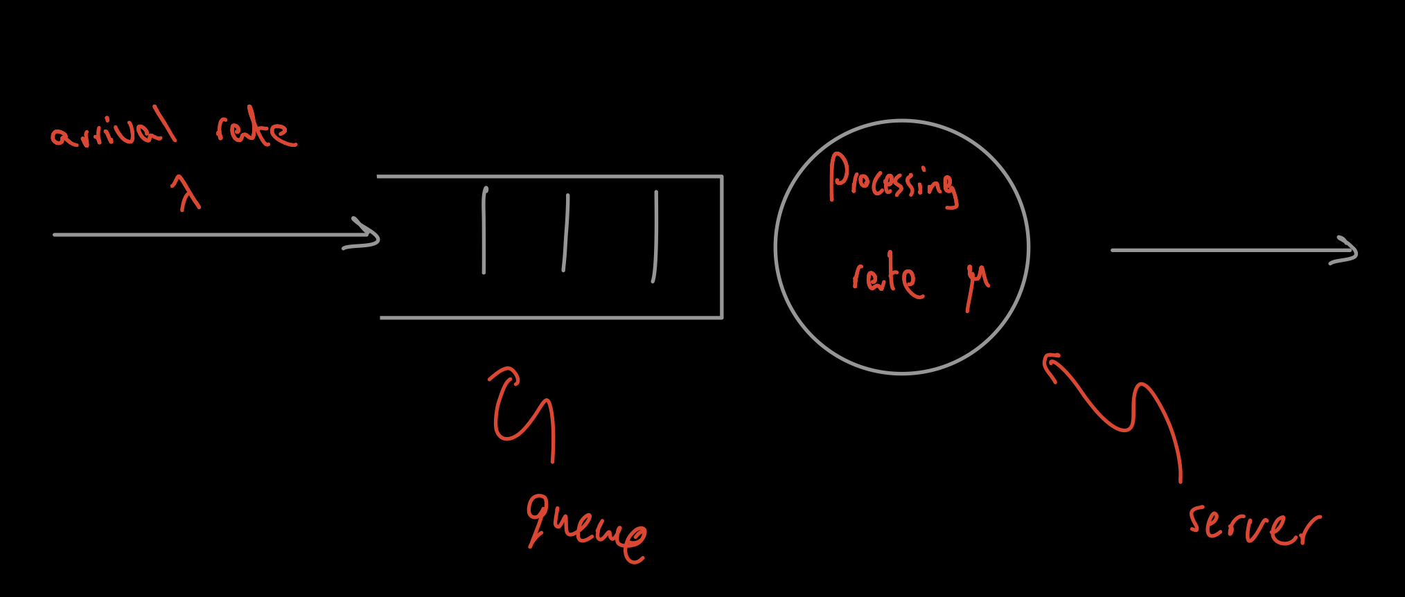
Queueing systems are modelled using Kendall’s notation as graphically shown below,

A queueing system can be specified with,

1. Number of servers s

2. Number of buffer spaces or queues

3. Queueing fashion: LIFO (last in first out) or FIFO (first in first out).

4. Arrival process: $\lambda$ being the mean arrival rate.

5. Service time: $\frac{1}{\mu}$ is the average processing time of an arrival.

Kendall’s Notation

Written as $M/M/s/k$. The first $M$ is inter-arrival time of processes, and denotes memoryless or exponential. The second $M$ is the service time and means a memoryless or exponential rate. $s$ is the number of servers as noted above, with $k$ being the total number of jobs in the server and buffer ($k-1$ is number of jobs in the buffer alone).

In general, rates are specified with symbols:

1. $M$: memoryless arrival or service times.

2. $G$: general arrival or service times.

3. $GI$: general and independent arrival or service time.

4. $D$: deterministic/constant arrival or service time.

Important properities of Poisson processes (exponentially distributed R.V.) for queueing systems:

1. $N_1(t)$ and $N_2(t)$ are independent Poisson processes with $\lambda_1$ and $\lambda_2$ parameters. Then $N_1(t) + N_2(t)$ is a Poisson process with parameter $\lambda_1 + \lambda_2$.

2. For Poisson process $N(t)$, when there’s an arrival, we can assign it to sub-process $N_k(t)$ with probability $p_k$, then we can generate $k$ random process $N_1(t), \cdots, N_k(t)$ with parameters $\lambda p_1, \cdots, \lambda p_k$ with $\sum\limits_{k=1}^K p_k = 1$.

Little’s Law

Let $W$ be the mean processing delay of a job, with $\lambda$ being the arrival rate. Then Little’s law gives the mean number of jobs in the system $L$ as, $$ L = \lambda W $$

$M/M/1$ Queue

This model is also called $M/M/1/\infty$. Since the system has exponential arrival rate, the queue is a continuous-time Markov chain (CTMC), with the following birth-death process,

The rate transition matrix $Q_{ij}$ from state $i$ to $j$ is,

$$ Q_{ij} = \begin{cases} &\lambda \hspace{1em} \text{, if } j = i + 1\\ & \mu \hspace{1em} \text{, if } j = i - 1\\ &-\lambda - \mu \hspace{1em} \text{, if } j = i \\ & 0 \hspace{1em} \text{, otherwise} \end{cases} $$

$\pi_n$ is the steady-state probability that there are n jobs in the system. Define $\rho = \frac{\lambda}{\mu}$, then solving the local-balance equations yields,

$$ \begin{aligned}& \lambda \pi_n = \mu \pi_{n+1} \\ & \pi_1 = \rho \pi_0 \\& \pi_2 = \rho \pi_1 = \rho^2 \pi_0 \\ & \hspace{1cm} \vdots \\ &\pi_n = \rho \pi_{n-1} = \rho^n \pi_0\end{aligned} $$

Since $\sum\limits_{n=0}^{\infty} \pi_n = 1$, then $\pi_0 \sum\limits_{n=0}^{\infty} \rho^n = 1$. With $\rho < 1$ to ensure that the service rate $\mu$ is higher than the arrival rate $\lambda$ (ensures system stability), the geometric sum is $\sum\limits_{n=0}^{\infty}\rho^n = \frac{1}{1-\rho}$. Then we have the stationary probability, $$ \pi_n = \rho^n (1 - \rho) $$

Note: The sum $\sum\limits_{n=0}^\infty \pi_n = 1$, since $\rho^n (1 - \rho)$, we have $(1 - \rho)\sum\limits_{n=0}^{\infty}\rho^n = \frac{1 - \rho}{1 - \rho} = 1 = \sum\limits_{n=0}^\infty \pi_n$. Meaning that the sum of stationary probabilities satisfies the normalization axiom of a probability distribution.

Waiting time and number of jobs

Mean number of jobs is $L := \sum\limits_{n=0}^{\infty} n \pi_n = \frac{\rho}{1-\rho}$. Mean delay or waiting time in the queue and service is $W = \frac{L}{\lambda} = \frac{1}{\mu - \lambda}$.

These expressions define the terms for being in the queue and the server.

For the queue-only values, define the mean waiting time in the queue as $W_q = W - \frac{1}{\mu} = \frac{\rho}{\mu - \lambda}$.

Mean number of customers in the queue is $L_q = \lambda W_q = \frac{\rho^2}{1 - \rho}$.

The mean server utilization is $U \triangleq 1 - \pi_0 = \rho$.